First Come First Serve(FCFS) Scheduling Algorithm in operating system
The simplest operating system scheduling method is thought to be FCFS. The first process to request a CPU is given that CPU first, according to the first come, first serve scheduling algorithm, which is implemented using a FIFO queue.
Characteristics of FCFS:
- Both non-preemptive and preemptive CPU scheduling techniques are supported by FCFS.
- It is always first-come, first-served while completing tasks.
- FCFS is simple to use and implement.
- The performance of this method is not very good, and the wait time is pretty long.
Advantages of FCFS:
- Easy to implement
- Method of “first come, first served”
Disadvantages of FCFS
- FCFS experiences the Convoy effect.
- Compared to other algorithms, the average waiting time is significantly longer.
- Consequently, FCFS is not very effective because it is so basic and straightforward to apply.
| Process | Arrival Time | Execution Time | Service Time |
| PO | 0 | 5 | 0 |
| P1 | 1 | 3 | 5 |
| P2 | 2 | 8 | 8 |
| P3 | 3 | 6 | 16 |
| 0 P0 5 | P1 8 | P2 16 | P3 22 |
|
Average Wait Time: (0+4+6+13) / 4 = 5.75
Example: Consider the following table, which provides adequate illustrations of the arrival time and burst time for the three processes P1, P2, and P3. The processes arrive at the location where they will be executed in the same way that is depicted in the table.
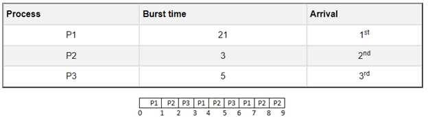
This is the chart of the above process
The average waiting time or AWT= (0+21+24)/3= 15ms
Firstly the process P1 will be executed by the CPU as its arrival time is 0.
So, there is no waiting time for the process P1 as CPU sits idle during this time.
The burst time of the process P1 is 21ms. So, it will take 21ms to complete its execution.
Thus, the time will be counted as waiting time for process P2.
In the same way, the waiting time for the process P3 can be calculated when we add the execution time of both the processes P1 and P2 i.e. waiting time for the process P3= 21+3=24 ms
Following the same procedure, the waiting time for the process P4= execution time of P1+P2+P3= 21+3+5= 29ms
So, we can completely explained this process through the chart which is illustrated above.
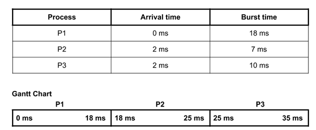
You can see from the sample above that there are three processes—P1, P2, and P3—and that they arrive in the ready state at 0 milliseconds, 2 milliseconds, and 2 milliseconds, respectively.
Therefore, the process P1 will be run for the first 18ms based on the arrival time. The process P2 will then run for 7 milliseconds, followed by the process P3, which will run for 10 milliseconds. One thing to keep in mind is that the CPU can choose any process if the processes’ arrival times are equal
| Process | Waiting Time | Turnaround Time |
———————————————
| P1 | 0ms | 18ms |
| P2 | 16ms | 23ms |
| P3 | 23ms | 33ms |
Total waiting time: (0 + 16 + 23) = 39ms
Average waiting time: (39/3) = 13ms
Total turnaround time: (18 + 23 + 33) = 74ms
Average turnaround time: (74/3) = 24.66ms