Lab4

Activity Outcomes:

This lab teaches you the following topics:

Introduction:

In the previous lab we studied breadth first search, which is the most naïve way of searching trees. The path returned by breadth search is not optimal. Uniform cost search always returns the optimal path. In this lab students will be able to implement a uniform cost search approach. Students will also be able to apply depth first search to their problems.

Lab Activities:

Activity 1:

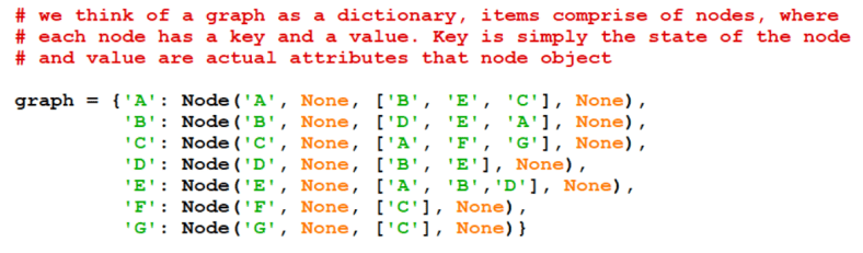
Consider a toy problem that can be represented as a following graph. How would you represent this graph in python?

Solution:

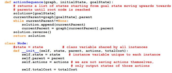
Remember a node of a tree can be represented by four attributes. We consider node as a class having four attributes namely,

• State of the node
• Parent of the node
• Actions applicable to that node (In the book/theory class, this attribute referred to the parent action that generated current node, however in this lab we will use this attribute to refer to all possible children states that are achievable from current state).
• The total path cost of that node starting from the initial state until that particular node is reached.

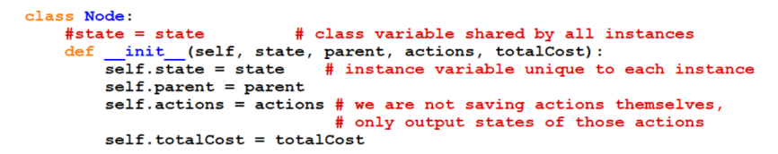
We can now implement this class in a dictionary. This dictionary will represent our state space graph. As we will traverse through the graph, we will keep updating parent and cost of each node.

Activity 2:

For the graph in previous activity, imagine node A as starting node and your goal is to reach F. Keeping depth first search in mind, describe a sequence of actions that you must take to reach that goal state.

Solution:

Remember that we can implement depth first search simply by using LIFO approach instead of FIFO that was used in breadth first search. Additionally we also don’t keep leaf nodes (nodes without children) in explored set.

Now the function definition is complete which can be called as follows,

Notice the difference in two portions of the code between breadth first search and depth first search. In the first we just pop out the last entry from the queue and in the 2nd difference we delete leaf nodes from the graph.

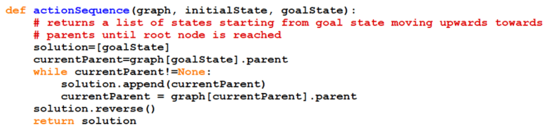
Calling DFS() will return the following solution,

Activity 3:

Change initial state to D and set goal state as C. What will be resulting path of BFS search? What will be the sequence of nodes explored?

Solution:

Final path is [‘D’, ‘B’, ‘A’, ‘C’]
Explored node sequence is D, E, A.

Activity 4:

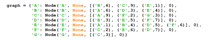
Imagine the same tree but this time we also mention the cost of each edge.

Implement a uniform cost solution to find the path from C to B.

Solution:

First we modify our graph structure so that in Node. actions is an array of tuples where each tuple contains a vertex and its associated weight.

We also modify the frontier format which will now be a dictionary. This dictionary will contain each node (the state of the node will act as a key and its parent and accumulated cost from the initial state will be two attributes of a particular key).
We now define a function which will give the node/key for which the cost is minimum. This will be implementation of pop method from the priority queue.

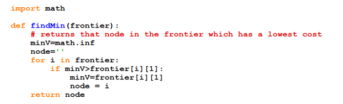
The rest of the functions are the same as in BFS i.e.,

Finally we define UCS()

solution = UCS()
print(solution)

The above two lines will print
[‘C’, ‘F’, ‘D’, ‘B’]

Home Activities:

Activity 1:

Imagine going from Arad to Bucharest in the following map. Your goal is to minimize the distance mentioned in the map during your travel. Implement a uniform cost search to find the corresponding path.